Areal Interpolation • duckspatial

This vignette demonstrates how to use ddbs_interpolate_aw() to perform areal-weighted interpolation. This technique is essential when you need to transfer attributes from one set of polygons (source) to another incongruent set of polygons (target) based on their area of overlap.

ddbs_interpolate_aw() can be 9-30x faster than sf::st_interpolate_aw or areal::aw_interpolate (see benchmarks in {ducksf} where prototype of ddbs_interpolate_aw() was originally developed).

duckspatial handles these heavy geometric calculations efficiently using DuckDB. We will cover three scenarios:

Extensive vs. Intensive: Understanding the difference between mass-preserving counts and densities.
Fast Output: Returning a tibble (no geometry) for maximum speed.
Database Mode: Performing operations on persistent database tables.

Setup Data

We will use the North Carolina dataset from the sf package as our source, and create a generic grid as our target.

Note: We project the data to Albers Equal Area (EPSG:5070) because accurate interpolation requires an equal-area projection.

library(duckspatial)
library(sf)

# 1. Load Source Data (NC Counties)
nc <- st_read(system.file("shape/nc.shp", package = "sf"), quiet = TRUE)

# 2. Transform to projected CRS (Albers) for accurate area calculations
nc <- st_transform(nc, 5070)

# 3. Create a Target Grid
grid <- st_make_grid(nc, n = c(10, 5)) |> st_as_sf()

# 4. Create Unique IDs (Required for interpolation)
nc$source_id <- 1:nrow(nc)
grid$target_id <- 1:nrow(grid)

1) Extensive vs. Intensive Interpolation

Areal interpolation works differently depending on the nature of the data.

Case A: Extensive Variables (Counts)

Variables like population counts or total births (BIR74) are spatially extensive. If a source polygon is split in half, the count should also be split in half. We use weight = "total" to ensure strict mass preservation relative to the source.

# Interpolate Total Births (Extensive)
res_extensive <- ddbs_interpolate_aw(
  target = grid,
  source = nc,
  tid = "target_id",
  sid = "source_id",
  extensive = "BIR74",
  weight = "total",
  output = "sf"
)
#> ✔ Query successful

Verification: The total sum of births in the result should match the original data (mass preservation).

orig_sum <- sum(nc$BIR74)
new_sum  <- sum(res_extensive$BIR74, na.rm = TRUE)

sprintf("Original: %s | Interpolated: %s", orig_sum, round(new_sum, 1))
#> [1] "Original: 329962 | Interpolated: 329962"

Case B: Intensive Variables (Densities/Ratios)

Variables like population density or infection rates are spatially intensive. If a source polygon is split, the density remains the same in both pieces. duckspatial handles this by calculating the area-weighted average.

# Interpolate 'BIR74' treating it as an intensive variable (e.g. density assumption)
res_intensive <- ddbs_interpolate_aw(
  target = grid,
  source = nc,
  tid = "target_id",
  sid = "source_id",
  intensive = "BIR74", # Treated as density here
  weight = "sum",      # Standard behavior for intensive vars
  output = "sf"
)
#> ✔ Query successful

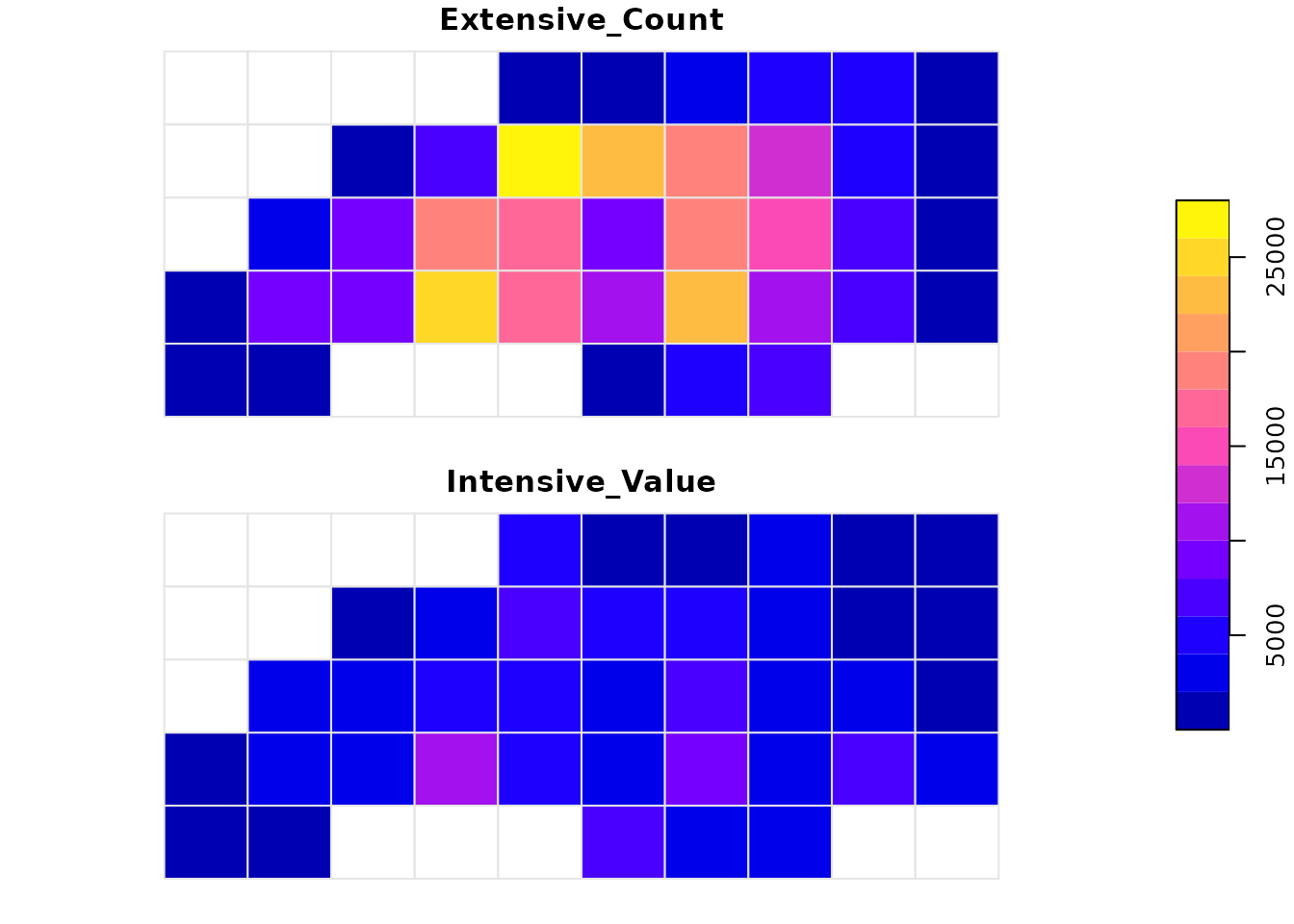
Visual Comparison

Notice the difference in patterns. Extensive interpolation accumulates values based on how much “stuff” falls into a grid cell, while intensive interpolation smoothes the values based on overlap.

# Combine for plotting
plot_data <- res_extensive[, "BIR74"]
names(plot_data)[1] <- "Extensive_Count"
plot_data$Intensive_Value <- res_intensive$BIR74

plot(plot_data[c("Extensive_Count", "Intensive_Value")], 
     main = "Interpolation Methods Comparison",
     border = "grey90",
     key.pos = 4)

2) High Performance: Output as Tibble

If you are working with massive datasets, constructing the geometry for the result sf object can be slow. If you only need the interpolated numbers, set output = "tibble". This skips the geometry construction step and is significantly faster.

# Return a standard data.frame/tibble without geometry
res_tbl <- ddbs_interpolate_aw(
  target = grid,
  source = nc,
  tid = "target_id",
  sid = "source_id",
  extensive = "BIR74",
  output = "tibble"
)
#> ✔ Query successful

head(res_tbl)
#> # A tibble: 6 × 3
#>   target_id crs_duckspatial BIR74
#>       <int> <chr>           <dbl>
#> 1         1 EPSG:5070       1168.
#> 2         2 EPSG:5070        379.
#> 3         6 EPSG:5070        753.
#> 4         7 EPSG:5070       5731.
#> 5         8 EPSG:5070       8000.
#> 6        11 EPSG:5070       1417.

3) Database Mode: Large Data Workflows

For datasets larger than memory, or for persistent pipelines, you can perform the interpolation directly inside the DuckDB database without pulling data into R until the end.

First, let’s establish a connection and load our spatial layers into tables.

# Create connection
conn <- ddbs_create_conn()

# Write layers to DuckDB
ddbs_write_vector(conn, nc, "nc_table", overwrite = TRUE)
#> Warning: `ddbs_write_vector()` was deprecated in duckspatial 1.0.0.
#> ℹ Please use `ddbs_write_table()` instead.
#> ℹ Table <nc_table> dropped
#> ✔ Table nc_table successfully imported
ddbs_write_vector(conn, grid, "grid_table", overwrite = TRUE)
#> ℹ Table <grid_table> dropped
#> ✔ Table grid_table successfully imported

Now we run the interpolation by referencing the table names. We can also use the name argument to save the result directly to a new table instead of returning it to R.

# Run interpolation and save to new table 'nc_grid_births'
ddbs_interpolate_aw(
  conn = conn,
  target = "grid_table",
  source = "nc_table",
  tid = "target_id",
  sid = "source_id",
  extensive = "BIR74",
  weight = "total",
  name = "nc_grid_births", # <--- Writes to DB
  overwrite = TRUE
)
#> ℹ Table <nc_grid_births> dropped
#> ✔ Query successful

# Verify the table was created
DBI::dbListTables(conn)
#> [1] "grid_table"     "nc_grid_births" "nc_table"

We can now query this table or read it back later.

# Read the result back from the database
final_sf <- ddbs_read_vector(conn, "nc_grid_births")
#> Warning: `ddbs_read_vector()` was deprecated in duckspatial 1.0.0.
#> ℹ Please use `ddbs_read_table()` instead.
#> ✔ table nc_grid_births successfully imported.

head(final_sf)
#> Simple feature collection with 6 features and 2 fields
#> Geometry type: POLYGON
#> Dimension:     XY
#> Bounding box:  xmin: 1054293 ymin: 1348021 xmax: 1677656 ymax: 1484503
#> Projected CRS: NAD83 / Conus Albers
#>   target_id     BIR74                              x
#> 1         1 1168.3093 POLYGON ((1054293 1348021, ...
#> 2         2  378.5281 POLYGON ((1132214 1348021, ...
#> 3         6  752.9156 POLYGON ((1443895 1348021, ...
#> 4         7 5731.0103 POLYGON ((1521815 1348021, ...
#> 5         8 7999.6957 POLYGON ((1599735 1348021, ...
#> 6        11 1416.5579 POLYGON ((1054293 1416262, ...

If we only wanted the database table, without the geometry, we could do:

ddbs_interpolate_aw(
  conn = conn,
  target = "grid_table",
  source = "nc_table",
  tid = "target_id",
  sid = "source_id",
  extensive = "BIR74",
  weight = "total",
  name = "nc_grid_births", # <--- Writes to DB
  overwrite = TRUE,
  output = "tibble"
)
#> ℹ Table <nc_grid_births> dropped
#> ✔ Query successful

And preview this table directly in the database:

DBI::dbGetQuery(conn, "SELECT * FROM nc_grid_births LIMIT 5")
#>   target_id crs_duckspatial     BIR74
#> 1         1       EPSG:5070 1168.3093
#> 2         2       EPSG:5070  378.5281
#> 3         6       EPSG:5070  752.9156
#> 4         7       EPSG:5070 5731.0103
#> 5         8       EPSG:5070 7999.6957

Cleanup

Always close the connection when finished.

duckdb::dbDisconnect(conn)