This vignette benchmarks {duckspatial} against {sf} across several spatial operations, comparing computation time and memory usage as dataset size grows. We plan to extend it with additional operation types in future releases. Versions of packages used in this vignette:
duckspatial: v1.0.0
duckdb: v1.5.1
sf: v1.1.0
TL;DR
{duckspatial} is substantially faster and allocates far less memory than {sf} in almost all cases, with the advantage becoming more pronounced on larger datasets. The one exception is pairwise distance calculation, where {sf} retains a memory advantage for Euclidean distances.
Prepare data
We are going to test the speed of a a bunch of functions using simulated data. We use the make_points() function to generate n random points within the globe, and 10,000 random rectangles.
Set-up
# Load necessary packages
library(duckspatial)
library(bench)
library(dplyr)
library(sf)
library(ggplot2)
options(scipen = 999)

# Function to generate random points
make_points <- function(n_points) {
    points_df <- data.frame(
      id = 1:n_points,
      x = runif(n_points, min = -180, max = 180),
      y = runif(n_points, min = -90, max = 90),
      value = rnorm(n_points, mean = 100, sd = 15),
      category = sample(c("A", "B", "C", "D"), n_points, replace = TRUE)
  ) |>
    sf::st_as_sf(coords = c("x", "y"), crs = 4326)
}

# Generate datasets of different sizes
withr::with_seed(27, {
  points_sf_100k <- make_points(1e5)
  points_sf_1mi  <- make_points(1e6)
  points_sf_3mi  <- make_points(3e6)
})

# Generate polygons
# Create large polygon dataset (e.g., administrative regions, zones, etc.)
n_polygons <- 10000
polygons_list <- vector("list", n_polygons)

for(i in 1:n_polygons) {
  # Random center point with buffer from edges
  center_x <- runif(1, min = -170, max = 170)
  center_y <- runif(1, min = -80, max = 80)

  # Create simple rectangular polygons to avoid geometry issues
  width <- runif(1, min = 0.5, max = 3)
  height <- runif(1, min = 0.5, max = 3)

  # Create rectangle coordinates (must be closed: first point = last point)
  x_coords <- c(
    center_x - width/2,
    center_x + width/2,
    center_x + width/2,
    center_x - width/2,
    center_x - width/2  # Close the polygon
  )

  y_coords <- c(
    center_y - height/2,
    center_y - height/2,
    center_y + height/2,
    center_y + height/2,
    center_y - height/2  # Close the polygon
  )

  # Create polygon matrix
  coords <- cbind(x_coords, y_coords)

  # Create polygon (wrapped in list as required by st_polygon)
  polygons_list[[i]] <- st_polygon(list(coords))
}

polygons_sf <- st_sf(
  poly_id    = 1:n_polygons,
  region     = sample(c("North", "South", "East", "West"), n_polygons, replace = TRUE),
  population = sample(1000:1000000, n_polygons, replace = TRUE),
  geometry   = st_sfc(polygons_list, crs = 4326)
)
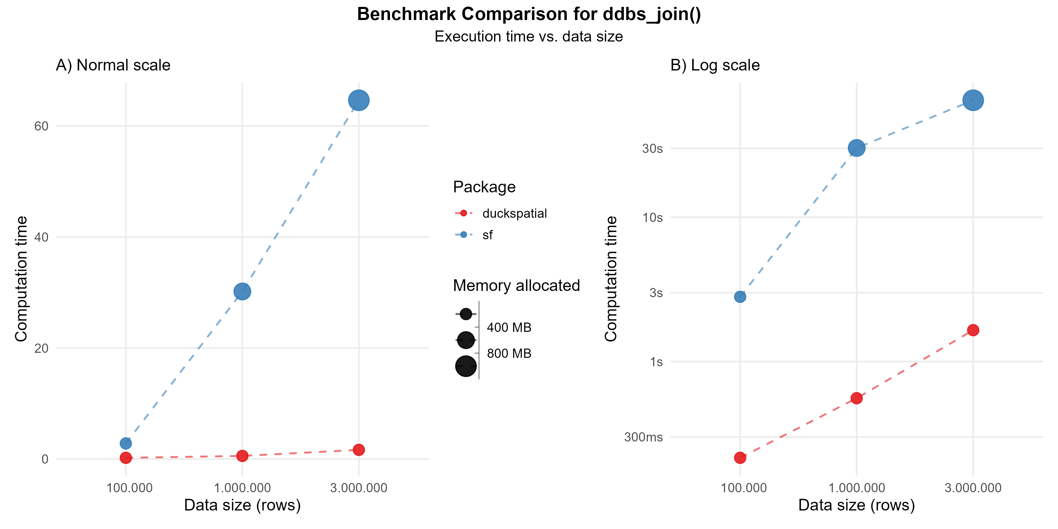
Spatial join
The spatial join aims to bring the attributes of a dataset to another dataset based in a spatial predicate. One example would be to have an x dataset with points that represent observations of wolves. In an y dataset, we could have polygons with attributes describing the geopraphical location (e.g. the name of the country, the name of the region..). So, by using a ST_Join(x, y, "intersects"), we would assign the attributes of y to x according to where the observation of the wolf fall.
This operation can be intensive. In the current version of {duckspatial} we see an improvement in speed and memory usage in bigger datasets, as shown in Figure 1.
Using 1 million points: {duckspatial} was about 50 times faster than {sf}, and allocated 18 times less memory.
Using 3 million points: {duckspatial} was about 35 times faster than {sf}, and allocated 16 times less memory.
Benchmark code - ddbs_join
# Helper to run the benchmark
run_join_benchmark <- function(points_sf) {
  temp <- bench::mark(
    iterations  = 3,
    check       = FALSE,
    duckspatial = ddbs_join(points_sf, polygons_sf, join = "within"),
    sf          = st_join(points_sf, polygons_sf, join = st_within)
  )
  temp$n   <- nrow(points_sf)
  temp$pkg <- c("duckspatial", "sf")
  temp
}

# Run the benchmark
df_bench_join <- lapply(
  X   = list(points_sf_100k, points_sf_1mi, points_sf_3mi),
  FUN = run_join_benchmark
) |>
  dplyr::bind_rows()
Spatial filter
The spatial filter aims to filter rows of x based in a spatial relationship with y. For example, let’s imagine that we have an x dataset with observations of wolves all around the world, and we want to filter only those that are in a specific country, for instance in Spain. If the dataset has this attritbute, we can just do it with a simple dplyr::filter(), but, if the wolves datase doesn’t include a column with the country, we can use a spatial filter. For that, we need a second dataset y with the boundaries of Spain, and by using ST_Filter(x, y, "intersects"), we would filter only those wolves observations that intersects with the Spain’s polygon.
In the current version of {duckspatial} we see an improvement in speed and memory usage in bigger datasets, as shown in Figure 2.
Using 1 million points: {duckspatial} was about 42 times faster than {sf}, and allocated 5 times less memory.
Using 3 million points: {duckspatial} was about 12 times faster than {sf}, and allocated 5 times less memory.
Benchmark code - ddbs_filter
# Helper to run the benchmark
run_filter_benchmark <- function(points_sf) {
  temp <- bench::mark(
    iterations  = 3,
    check       = FALSE,
    duckspatial = ddbs_filter(points_sf, polygons_sf),
    sf          = st_filter(points_sf, polygons_sf)
  )
  temp$n   <- nrow(points_sf)
  temp$pkg <- c("duckspatial", "sf")
  temp
}

# Run the benchmark
df_bench_filter <- lapply(
  X   = list(points_sf_100k, points_sf_1mi, points_sf_3mi),
  FUN = run_filter_benchmark
) |>
  dplyr::bind_rows()
Spatial distances
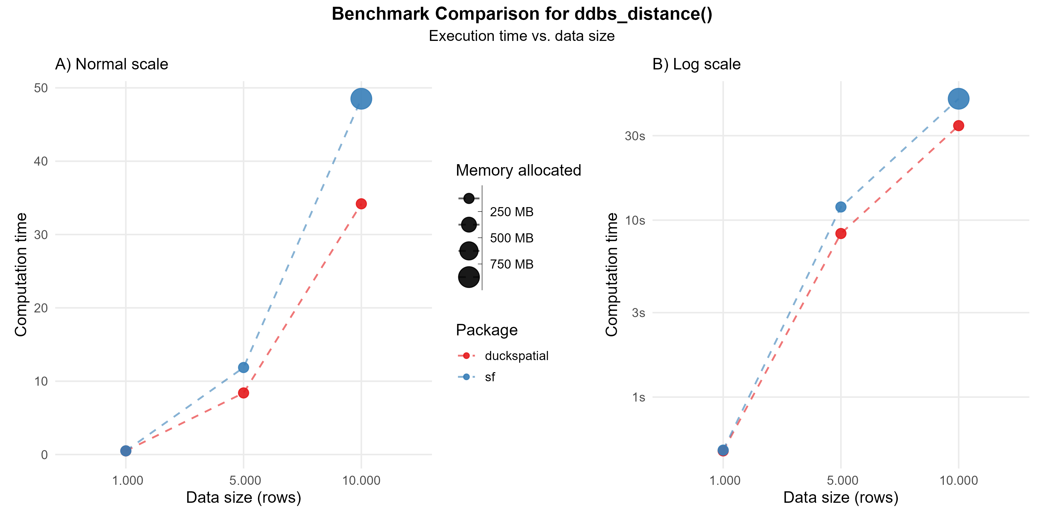
The ST_Distance(x, y) calculates the distance between each observation in x against each observation in y. The default {duckspatial} mode will return a lazy table with three columns: (id_x) the id of the row in x; (id_y) the id of the row in y; (distance) the actual distance between those pair of observations. In the case of mode = 'sf', the result will be a sparse matrix. Note that {duckspatial} will use by default the best distance for the input CRS and geometry type.
When calculating the distance between 10,000 pairs of points, {duckspatial} was about 1.5 times faster, but used much less memory (> 400 times).
Benchmark code - ddbs_distance
# Helper to run the benchmark
run_distance_benchmark <- function(n) {

  points_sf <- withr::with_seed(27, make_points(n))

  temp <- bench::mark(
    iterations  = 1,
    check       = FALSE,
    duckspatial = ddbs_distance(points_sf, points_sf),
    sf          = st_distance(points_sf, points_sf)
  )
  temp$n   <- n
  temp$pkg <- c("duckspatial", "sf")
  temp
}

df_bench_distance <- lapply(
  X   = c(1000, 5000, 10000),
  FUN = run_distance_benchmark
) |>
  dplyr::bind_rows()
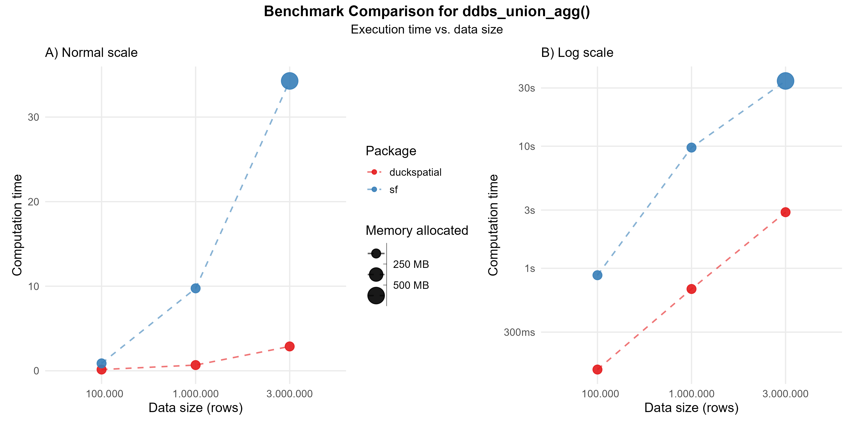
Dissolving geometries
Dissolving geometries consist in merging/aggregating geometries that share a common attribute into a single geometry per group.
In the current version of {duckspatial} we see an improvement in speed and memory usage in bigger datasets, as shown in Figure 4.
Using 1 million points: {duckspatial} was about 14 times faster than {sf}, and allocated 10 times less memory.
Using 3 million points: {duckspatial} was about 12 times faster than {sf}, and allocated 10 times less memory.
Benchmark code - ddbs_union_agg
# Helper to run the benchmark
run_union_benchmark <- function(points_sf) {
  temp <- bench::mark(
    iterations  = 3,
    check       = FALSE,
    duckspatial = ddbs_union_agg(points_sf, by = "category"),
    sf          = points_sf |>
      group_by(category) |>
      summarise(geometry = st_union(geometry))
  )
  temp$n   <- nrow(points_sf)
  temp$pkg <- c("duckspatial", "sf")
  temp
}

# Run the benchmark
df_bench_union <- lapply(
  X   = list(points_sf_100k, points_sf_1mi, points_sf_3mi),
  FUN = run_union_benchmark
) |>
  dplyr::bind_rows()
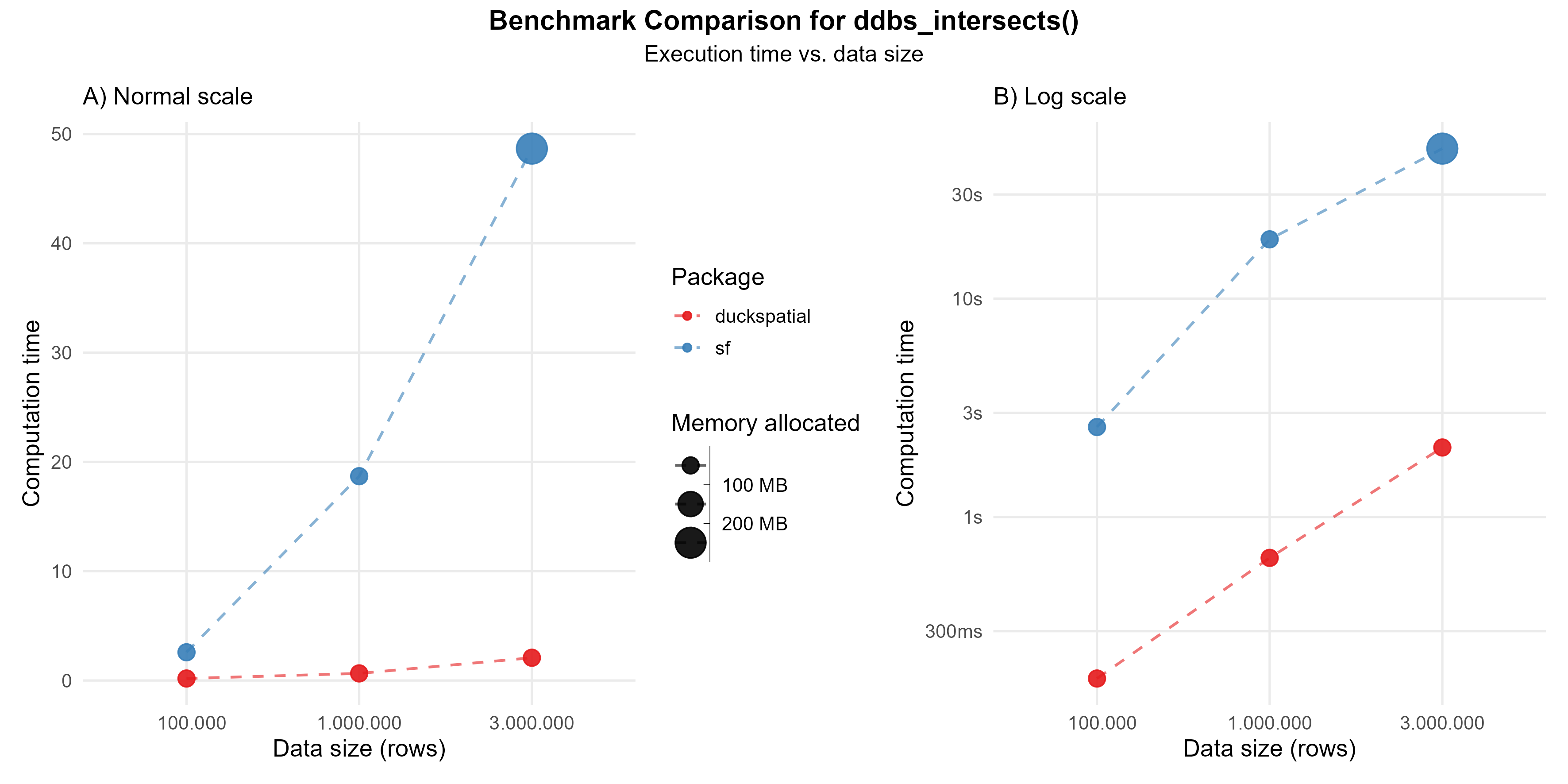
Geometry predicates
Geometry predicates are boolean functions that test spatial relationships between two geometries (they return true or false). They’re fundamental to spatial queries, letting you filter or join data based on how geometries relate to one another in space. Common examples include: ST_Contains, ST_Within, ST_Touches, ST_Overlaps, ST_Crosses, ST_Disjoint, and ST_Equals.
In the following example, we compare ST_Intersects(geometry A, geometry B), which returns true if the two geometries share any point in common (their interiors or boundaries overlap in any way).
Using 1 million points: {duckspatial} was about 28 times faster than {sf}, and allocated 3 times less memory.
Using 3 million points: {duckspatial} was about 23 times faster than {sf}, and allocated 3 times less memory.
Benchmark code - ddbs_intersects
# Helper to run the benchmark
run_predicate_benchmark <- function(points_sf) {
  temp <- bench::mark(
    iterations  = 1,
    check       = FALSE,
    duckspatial = ddbs_intersects(points_sf, polygons_sf),
    sf          = st_intersects(points_sf, polygons_sf)
  )
  temp$n   <- nrow(points_sf)
  temp$pkg <- c("duckspatial", "sf")
  temp
}

# Run the benchmark
df_bench_predicate <- lapply(
  X   = list(points_sf_100k, points_sf_1mi, points_sf_3mi),
  FUN = run_predicate_benchmark
) |>
  dplyr::bind_rows()